
Illustration by Paweł Jońca
In 2019, the Event Horizon Telescope team gave the world the first glimpse of what a black hole actually looks like. But the image of a glowing, ring-shaped object that the group unveiled wasn’t a conventional photograph. It was computed — a mathematical transformation of data captured by radio telescopes in the United States, Mexico, Chile, Spain and the South Pole1. The team released the programming code it used to accomplish that feat alongside the articles that documented its findings, so the scientific community could see — and build on — what it had done.
It’s an increasingly common pattern. From astronomy to zoology, behind every great scientific finding of the modern age, there is a computer. Michael Levitt, a computational biologist at Stanford University in California who won a share of the 2013 Nobel Prize in Chemistry for his work on computational strategies for modelling chemical structure, notes that today’s laptops have about 10,000 times the memory and clock speed that his lab-built computer had in 1967, when he began his prizewinning work. “We really do have quite phenomenal amounts of computing at our hands today,” he says. “Trouble is, it still requires thinking.”
Enter the scientist-coder. A powerful computer is useless without software capable of tackling research questions — and researchers who know how to write it and use it. “Research is now fundamentally connected to software,” says Neil Chue Hong, director of the Software Sustainability Institute, headquartered in Edinburgh, UK, an organization dedicated to improving the development and use of software in science. “It permeates every aspect of the conduct of research.”
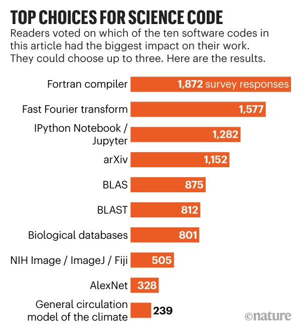
Scientific discoveries rightly get top billing in the media. But Nature this week looks behind the scenes, at the key pieces of code that have transformed research over the past few decades.
Although no list like this can be definitive, we polled dozens of researchers over the past year to develop a diverse line-up of ten software tools that have had a big impact on the world of science.
Language pioneer: the Fortran compiler (1957)
The first modern computers weren’t user-friendly. Programming was literally done by hand, by connecting banks of circuits with wires. Subsequent machine and assembly languages allowed users to program computers in code, but both still required an intimate knowledge of the computer’s architecture, putting the languages out of reach of many scientists.
That changed in the 1950s with the development of symbolic languages — in particular the ‘formula translation’ language Fortran, developed by John Backus and his team at IBM in San Jose, California. Using Fortran, users could program computers using human-readable instructions, such as x = 3 + 5. A compiler then turned such directions into fast, efficient machine code.
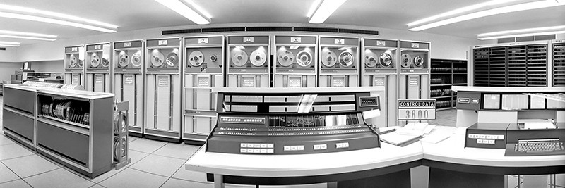
This CDC 3600 computer, delivered in 1963 to the National Center for Atmospheric Research in Boulder, Colorado, was programmed with the help of the Fortran compiler.Credit: University Corporation for Atmospheric Research/Science Photo Library
It still wasn’t easy: in the early days, programmers used punch cards to input code, and a complex simulation might require tens of thousands of them. Still, says Syukuro Manabe, a climatologist at Princeton University in New Jersey, Fortran made programming accessible to researchers who weren’t computer scientists. “For the first time, we were able to program [the computer] by ourselves,” Manabe says. He and his colleagues used the language to develop one of the first successful climate models.
Now in its eighth decade, Fortran is still widely used in climate modelling, fluid dynamics, computational chemistry — any discipline that involves complex linear algebra and requires powerful computers to crunch numbers quickly. The resulting code is fast, and there are still plenty of programmers who know how to write it. Vintage Fortran code bases are still alive and kicking in labs and on supercomputers worldwide. “Old-time programmers knew what they were doing,” says Frank Giraldo, an applied mathematician and climate modeller at the Naval Postgraduate School in Monterey, California. “They were very mindful of memory, because they had so little of it.”
Signal processor: fast Fourier transform (1965)
When radioastronomers scan the sky, they capture a cacophony of complex signals changing with time. To understand the nature of those radio waves, they need to see what those signals look like as a function of frequency. A mathematical process called a Fourier transform allows researchers to do that. The problem is that it’s inefficient, requiring N2 calculations for a data set of size N.
In 1965, US mathematicians James Cooley and John Tukey worked out a way to accelerate the process. Using recursion, a ‘divide and conquer’ programming approach in which an algorithm repeatedly reapplies itself, the fast Fourier transform (FFT) simplifies the problem of computing a Fourier transform to just N log2(N) steps. The speed improves as N grows. For 1,000 points, the speed boost is about 100-fold; for 1 million points, it’s 50,000-fold.
The ‘discovery’ was actually a rediscovery — the German mathematician Carl Friedrich Gauss worked it out in 1805, but he never published it, says Nick Trefethen, a mathematician at the University of Oxford, UK. But Cooley and Tukey did, opening applications in digital signal processing, image analysis, structural biology and more. “It’s really one of the great events in applied mathematics and engineering,” Trefethen says. FFT has been implemented many times in code. One popular option is called FFTW, the ‘fastest Fourier transform in the west’.

A night view of part of the Murchison Widefield Array, a radio telescope in Western Australia that uses fast Fourier transforms for data collection.Credit: John Goldsmith/Celestial Visions
Paul Adams, who directs the molecular biophysics and integrated bioimaging division at Lawrence Berkeley National Laboratory in California, recalls that when he refined the structure of the bacterial protein GroEL in 19952, the calculation took “many, many hours, if not days”, even with the FFT and a supercomputer. “Trying to do those without the FFT, I don’t even know how we would have done that realistically,” he says. “It would have just taken forever.”
Molecular cataloguers: biological databases (1965)
Databases are such a seamless component of scientific research today that it can be easy to overlook the fact that they are driven by software. In the past few decades, these resources have ballooned in size and shaped many fields, but perhaps nowhere has that transformation been more dramatic than in biology.
Today’s massive genome and protein databases have their roots in the work of Margaret Dayhoff, a bioinformatics pioneer at the National Biomedical Research Foundation in Silver Spring, Maryland. In the early 1960s, as biologists worked to tease apart proteins’ amino acid sequences, Dayhoff began collating that information in search of clues into evolutionary relationships between different species. Her Atlas of Protein Sequence and Structure, first published in 1965 with three co-authors, described what was then known of the sequences, structures and similarities of 65 proteins. The collection was the first that “was not tied to a specific research question”, historian Bruno Strasser wrote in 20103. And it encoded its data in punch cards, which made it possible to expand the database and search it.
Other computerized biological databases followed. The Protein Data Bank, which today details more than 170,000 macromolecular structures, went live in 1971. Russell Doolittle, an evolutionary biologist at the University of California, San Diego, created another protein database called Newat in 1981. And 1982 saw the release of the database that would become GenBank, the DNA archive maintained by the US National Institutes of Health.
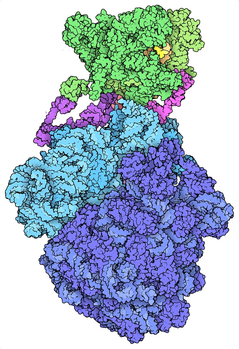
The Protein Data Bank has an archive of more than 170,000 molecular structures including this bacterial ‘expressome’, which combines the processes of RNA and protein synthesis.Credit: David S. Goodsell and RCSB PDB (CC BY 4.0)
Such resources proved their worth in July 1983, when separate teams led by Michael Waterfield, a protein biochemist at the Imperial Cancer Research Fund in London, and Doolittle independently reported a similarity between the sequences of a particular human growth factor and a protein in a virus that causes cancer in monkeys. The observation suggested a mechanism for oncogenesis-by-virus — that by mimicking a growth factor, the virus induces uncontrolled growth of cells4. “That set the light bulb off in some of the minds of biologists who were not into computers and statistics,” says James Ostell, former director of the US National Center for Biotechnology Information (NCBI): “We can understand something about cancer from comparing sequences.”
Beyond that, Ostell says, the discovery marked “an advent of objective biology”. In addition to designing experiments to test specific hypotheses, researchers could mine public data sets for connections that might never have occurred to those who actually collected the data. That power grows drastically when different data sets are linked together — something NCBI programmers achieved in 1991 with Entrez, a tool that allows researchers to freely navigate from DNA to protein to literature and back.
Stephen Sherry, current acting director of the NCBI in Bethesda, Maryland, used Entrez as a graduate student. “I remember at the time thinking it was magic,” he says.
Forecast leader: the general circulation model (1969)
At the close of the Second World War, computer pioneer John von Neumann began turning computers that a few years earlier had been calculating ballistics trajectories and weapon designs towards the problem of weather prediction. Up until that point, explains Manabe, “weather forecasting was just empirical”, using experience and hunches to predict what would happen next. Von Neumann’s team, by contrast, “attempted to do numerical weather prediction based upon laws of physics”.
The equations had been known for decades, says Venkatramani Balaji, head of the Modeling Systems Division at the National Oceanographic and Atmospheric Administration’s Geophysical Fluid Dynamics Laboratory in Princeton, New Jersey. But early meteorologists couldn’t solve them practically. To do so required inputting current conditions, calculating how they would change over a short time period, and repeating — a process so time-consuming that the mathematics couldn’t be completed before the weather itself caught up. In 1922, the mathematician Lewis Fry Richardson spent months crunching a six-hour forecast for Munich, Germany. The result, according to one history, was “wildly inaccurate”, including predictions that “could never occur under any known terrestrial conditions”. Computers made the problem tractable.
In the late 1940s, von Neumann established his weather-prediction team at the Institute for Advanced Study at Princeton. In 1955, a second team — the Geophysical Fluid Dynamics Laboratory — began work on what he called “the infinite forecast” — that is, climate modelling.
Manabe, who joined the climate modelling team in 1958, set to work on atmospheric models; his colleague Kirk Bryan addressed those for the ocean. In 1969, they successfully combined the two, creating what Nature in 2006 called a “milestone” in scientific computing.
Today’s models can divide the planet’s surface into squares measuring 25 × 25 kilometres, and the atmosphere into dozens of levels. By contrast, Manabe and…